Linear systems solution algebraic equations(SLAE) is undoubtedly the most important topic of the linear algebra course. Great amount problems from all branches of mathematics is reduced to solving systems linear equations... These factors explain the reason for creating this article. The material of the article is selected and structured so that with its help you can

• choose the optimal method for solving your system of linear algebraic equations,
• study the theory of the chosen method,
• solve your system of linear equations by considering detailed solutions typical examples and tasks.

Brief description of the article material.

First, we give all the necessary definitions and concepts and introduce the notation.

Next, we will consider methods for solving systems of linear algebraic equations in which the number of equations is equal to the number of unknown variables and which have a unique solution. First, let us dwell on Cramer's method, secondly, show a matrix method for solving such systems of equations, and thirdly, analyze the Gauss method (the method of successive elimination of unknown variables). To consolidate the theory, we will definitely solve several SLAEs in different ways.

After that, we turn to solving systems of linear algebraic equations of general form, in which the number of equations does not coincide with the number of unknown variables or the main matrix of the system is degenerate. Let us formulate the Kronecker - Capelli theorem, which allows us to establish the compatibility of SLAEs. Let us analyze the solution of systems (in the case of their compatibility) using the concept of a basic minor of a matrix. We will also consider the Gaussian method and describe in detail the solutions of examples.

We will definitely dwell on the structure of the general solution of homogeneous and inhomogeneous systems of linear algebraic equations. Let us give the concept of a fundamental system of solutions and show how the general solution of an SLAE is written using vectors of the fundamental system of solutions. For a better understanding, let's look at a few examples.

In conclusion, we consider systems of equations that reduce to linear ones, as well as various problems, in the solution of which SLAEs arise.

Page navigation.

Definitions, concepts, designations.

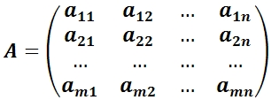
We will consider systems of p linear algebraic equations with n unknown variables (p can be equal to n) of the form

Unknown variables, - coefficients (some real or complex numbers), - free members (also real or complex numbers).

This form of SLAE notation is called coordinate.

V matrix form notation, this system of equations has the form,
where - the main matrix of the system, - the matrix-column of unknown variables, - the matrix-column of free members.

If to the matrix A we add as the (n + 1) th column the matrix-column of free terms, then we get the so-called expanded matrix systems of linear equations. Usually, the expanded matrix is ​​denoted by the letter T, and the column of free members is separated by a vertical line from the rest of the columns, that is,

By solving a system of linear algebraic equations is a set of values ​​of unknown variables that converts all equations of the system into identities. The matrix equation for the given values ​​of the unknown variables also turns into an identity.

If a system of equations has at least one solution, then it is called joint.

If the system of equations has no solutions, then it is called inconsistent.

If the SLAE has a unique solution, then it is called certain; if there is more than one solution, then - undefined.

If the free terms of all equations of the system are equal to zero , then the system is called homogeneous, otherwise - heterogeneous.

Solution of elementary systems of linear algebraic equations.

If the number of equations of the system is equal to the number of unknown variables and the determinant of its main matrix is ​​not equal to zero, then such SLAEs will be called elementary... Such systems of equations have a unique solution, and in the case of a homogeneous system, all unknown variables are equal to zero.

We began to study such SLAEs in high school. When solving them, we took one equation, expressed one unknown variable in terms of others and substituted it into the remaining equations, then we took the next equation, expressed the next unknown variable and substituted it into other equations, and so on. Or they used the method of addition, that is, they added two or more equations to eliminate some unknown variables. We will not dwell on these methods in detail, since they are, in fact, modifications of the Gauss method.

The main methods for solving elementary systems of linear equations are the Cramer method, the matrix method and the Gauss method. Let's analyze them.

Solving systems of linear equations by Cramer's method.

Suppose we need to solve a system of linear algebraic equations

in which the number of equations is equal to the number of unknown variables and the determinant of the main matrix of the system is nonzero, that is,.

Let be the determinant of the main matrix of the system, and - determinants of matrices, which are obtained from A by replacing 1st, 2nd, ..., nth column, respectively, to the column of free members:

With this notation, the unknown variables are calculated by the formulas of Cramer's method as ... This is how the solution of a system of linear algebraic equations by Cramer's method is found.

Example.

Cramer's method .

Solution.

The main matrix of the system has the form ... Let's calculate its determinant (if necessary, see the article):

Since the determinant of the main matrix of the system is nonzero, the system has a unique solution that can be found by Cramer's method.

Let us compose and calculate the necessary determinants (the determinant is obtained by replacing the first column in matrix A with a column of free members, the determinant - by replacing the second column with a column of free members, - by replacing the third column of matrix A with a column of free members):

Find unknown variables by the formulas :

Answer:

The main drawback of Cramer's method (if it can be called a drawback) is the complexity of calculating determinants when the number of equations in the system is more than three.

Solving systems of linear algebraic equations by the matrix method (using the inverse matrix).

Let the system of linear algebraic equations be given in matrix form, where matrix A has dimension n by n and its determinant is nonzero.

Since, the matrix A is invertible, that is, there is an inverse matrix. If we multiply both sides of the equality by the left, then we get a formula for finding the column matrix of unknown variables. So we got the solution of a system of linear algebraic equations by the matrix method.

Example.

Solve a system of linear equations matrix method.

Solution.

Let's rewrite the system of equations in matrix form:

Because

then SLAE can be solved by the matrix method. By using inverse matrix the solution to this system can be found as .

Let's construct an inverse matrix using a matrix of algebraic complements of elements of matrix A (if necessary, see the article):

It remains to calculate - the matrix of unknown variables by multiplying the inverse matrix to a column matrix of free members (see the article if necessary):

Answer:

or in another notation x 1 = 4, x 2 = 0, x 3 = -1.

The main problem in finding a solution to systems of linear algebraic equations by the matrix method is the complexity of finding the inverse matrix, especially for square matrices of order higher than the third.

Solution of systems of linear equations by the Gauss method.

Suppose we need to find a solution to a system of n linear equations with n unknown variables
the determinant of the main matrix of which is nonzero.

The essence of the Gauss method consists in the successive elimination of unknown variables: first, x 1 is excluded from all equations of the system, starting with the second, then x 2 is excluded from all equations, starting with the third, and so on, until only the unknown variable x n remains in the last equation. Such a process of transforming the equations of the system for the successive elimination of unknown variables is called by the direct course of the Gauss method... After completing the forward run of the Gauss method, x n is found from the last equation, using this value, x n-1 is calculated from the penultimate equation, and so on, x 1 is found from the first equation. The process of calculating unknown variables when moving from the last equation of the system to the first is called backward Gaussian method.

Let us briefly describe the algorithm for eliminating unknown variables.

We will assume that, since we can always achieve this by rearranging the equations of the system. Eliminate the unknown variable x 1 from all equations of the system, starting with the second. To do this, to the second equation of the system we add the first, multiplied by, to the third equation we add the first, multiplied by, and so on, to the n-th equation we add the first, multiplied by. The system of equations after such transformations takes the form

where, and .

We would come to the same result if we expressed x 1 in terms of other unknown variables in the first equation of the system and substituted the resulting expression in all other equations. Thus, the variable x 1 is excluded from all equations, starting with the second.

Next, we act in a similar way, but only with a part of the resulting system, which is marked in the figure

To do this, to the third equation of the system we add the second multiplied by, to the fourth equation we add the second multiplied by, and so on, to the n-th equation we add the second multiplied by. The system of equations after such transformations takes the form

where, and ... Thus, the variable x 2 is excluded from all equations, starting with the third.

Next, we proceed to the elimination of the unknown x 3, while we act similarly with the part of the system marked in the figure

So we continue the direct course of the Gauss method until the system takes the form

From this moment we begin reverse Gauss method: we calculate x n from the last equation as, using the obtained value of x n, we find x n-1 from the penultimate equation, and so on, we find x 1 from the first equation.

Example.

Solve a system of linear equations by the Gauss method.

Solution.

Eliminate the unknown variable x 1 from the second and third equations of the system. To do this, add to both parts of the second and third equations the corresponding parts of the first equation, multiplied by and by, respectively:

Now we exclude x 2 from the third equation by adding to its left and right sides the left and right sides of the second equation, multiplied by:

At this point, the forward move of the Gauss method is over, we begin the reverse move.

From the last equation of the resulting system of equations, we find x 3:

From the second equation we get.

From the first equation, we find the remaining unknown variable and this completes the reverse course of the Gauss method.

Answer:

X 1 = 4, x 2 = 0, x 3 = -1.

Solution of systems of linear algebraic equations of general form.

In the general case, the number of equations in the system p does not coincide with the number of unknown variables n:

Such SLAEs may have no solutions, have a single solution, or have infinitely many solutions. This statement also applies to systems of equations, the basic matrix of which is square and degenerate.

The Kronecker - Capelli theorem.

Before finding a solution to a system of linear equations, it is necessary to establish its compatibility. The answer to the question when the SLAE is compatible and when it is incompatible is given by the Kronecker - Capelli theorem:
for a system of p equations with n unknowns (p can be equal to n) to be consistent, it is necessary and sufficient that the rank of the main matrix of the system be equal to the rank of the extended matrix, that is, Rank (A) = Rank (T).

Let us consider by example the application of the Kronecker - Capelli theorem to determine the compatibility of a system of linear equations.

Example.

Find out if the system of linear equations solutions.

Solution.

... Let's use the bordering minors method. Minor of the second order nonzero. Let's sort out the third-order minors bordering it:

Since all bordering minors of the third order are equal to zero, the rank of the main matrix is ​​equal to two.

In turn, the rank of the extended matrix is equal to three, since the third-order minor

nonzero.

Thus, Rang (A), therefore, by the Kronecker - Capelli theorem, we can conclude that the original system of linear equations is inconsistent.

Answer:

The system has no solutions.

So, we have learned to establish the inconsistency of the system using the Kronecker - Capelli theorem.

But how to find a solution to a SLAE if its compatibility has been established?

To do this, we need the concept of a basic minor of a matrix and a theorem on the rank of a matrix.

Minor highest order matrix A, different from zero, is called basic.

It follows from the definition of a basic minor that its order is equal to the rank of the matrix. For a nonzero matrix A, there can be several basic minors; there is always one basic minor.

For example, consider the matrix .

All third-order minors of this matrix are equal to zero, since the elements of the third row of this matrix are the sum of the corresponding elements of the first and second rows.

The following second-order minors are basic, since they are nonzero

Minors are not basic, since they are equal to zero.

Matrix rank theorem.

If the rank of a matrix of order p by n is equal to r, then all elements of the rows (and columns) of the matrix that do not form the selected basic minor are linearly expressed in terms of the corresponding elements of the rows (and columns) that form the basic minor.

What does the matrix rank theorem give us?

If, by the Kronecker - Capelli theorem, we have established the compatibility of the system, then we choose any basic minor of the basic matrix of the system (its order is r), and we exclude from the system all equations that do not form the chosen basic minor. The SLAE obtained in this way will be equivalent to the original one, since the discarded equations are still superfluous (according to the matrix rank theorem, they are a linear combination of the remaining equations).

As a result, after discarding unnecessary equations of the system, two cases are possible.

If the number of equations r in the resulting system is equal to the number of unknown variables, then it will be definite and the only solution can be found by Cramer's method, matrix method or Gauss's method.

Example.

.

Solution.

The rank of the main matrix of the system is equal to two, since the second order minor nonzero. Extended Matrix Rank is also equal to two, since the only minor of the third order is equal to zero

and the second-order minor considered above is nonzero. Based on the Kronecker - Capelli theorem, we can assert the compatibility of the original system of linear equations, since Rank (A) = Rank (T) = 2.

We take as a basic minor ... It is formed by the coefficients of the first and second equations:


The third equation of the system does not participate in the formation of the basic minor; therefore, we exclude it from the system based on the theorem on the rank of the matrix:


This is how we got an elementary system of linear algebraic equations. Let's solve it using Cramer's method:


Answer:

x 1 = 1, x 2 = 2.

If the number of equations r in the obtained SLAE is less than the number of unknown variables n, then in the left-hand sides of the equations we leave the terms forming the basic minor, the remaining terms are transferred to the right-hand sides of the equations of the system with the opposite sign.

Unknown variables (there are r of them) remaining in the left-hand sides of the equations are called the main.

Unknown variables (there are n - r pieces) that appear in the right-hand sides are called free.

Now we assume that free unknown variables can take arbitrary values, while r basic unknown variables will be expressed in terms of free unknown variables in a unique way. Their expression can be found by solving the obtained SLAE by the Cramer method, by the matrix method, or by the Gaussian method.

Let's take an example.

Example.

Solve a system of linear algebraic equations .

Solution.

Find the rank of the main matrix of the system by the method of bordering minors. We take a 1 1 = 1 as a nonzero first-order minor. Let's start looking for a nonzero second-order minor that surrounds this minor:


This is how we found a nonzero second-order minor. Let's start looking for a third-order nonzero bordering minor:


Thus, the rank of the main matrix is ​​three. The rank of the extended matrix is ​​also three, that is, the system is consistent.

We take the found nonzero third-order minor as the basic one.

For clarity, we show the elements that form the basic minor:


We leave on the left side of the equations of the system the terms participating in the basic minor, the rest are transferred with opposite signs to the right sides:


Let us assign arbitrary values ​​to the free unknown variables x 2 and x 5, that is, we take , where are arbitrary numbers. In this case, the SLAE will take the form


The resulting elementary system of linear algebraic equations is solved by Cramer's method:


Hence, .

Do not forget to specify free unknown variables in your answer.

Answer:

Where are arbitrary numbers.

Summarize.

To solve a system of linear algebraic equations of general form, we first find out its compatibility using the Kronecker - Capelli theorem. If the rank of the main matrix is ​​not equal to the rank of the extended matrix, then we conclude that the system is incompatible.

If the rank of the main matrix is ​​equal to the rank of the extended matrix, then we choose the basic minor and discard the equations of the system that do not participate in the formation of the selected basic minor.

If the order of the basic minor is equal to the number unknown variables, then the SLAE has a unique solution that we find by any method known to us.

If the order of the basic minor is less than the number of unknown variables, then on the left-hand side of the equations of the system we leave the terms with the basic unknown variables, transfer the remaining terms to the right-hand sides and give arbitrary values ​​to the free unknown variables. From the resulting system of linear equations, we find the main unknown variables by the Cramer method, the matrix method, or the Gauss method.

Gauss method for solving systems of linear algebraic equations of general form.

The Gauss method can be used to solve systems of linear algebraic equations of any kind without first examining them for compatibility. The process of successive elimination of unknown variables makes it possible to conclude both the compatibility and the incompatibility of the SLAE, and if a solution exists, it makes it possible to find it.

From the point of view of computational work, the Gaussian method is preferable.

Watch it detailed description and discussed examples in the article the Gauss method for solving systems of linear algebraic equations of general form.

Writing the general solution of homogeneous and inhomogeneous linear algebraic systems using vectors of the fundamental system of solutions.

In this section, we will focus on compatible homogeneous and inhomogeneous systems of linear algebraic equations with an infinite set of solutions.

Let's deal first with homogeneous systems.

Fundamental decision system A homogeneous system of p linear algebraic equations with n unknown variables is the set (n - r) of linearly independent solutions of this system, where r is the order of the basic minor of the basic matrix of the system.

If we denote linearly independent solutions of a homogeneous SLAE as X (1), X (2),…, X (nr) (X (1), X (2),…, X (nr) are n-by-1 column matrices) , then the general solution of this homogeneous system is represented as a linear combination of vectors of the fundamental system of solutions with arbitrary constant coefficients С 1, С 2, ..., С (nr), that is,.

What does the term general solution of a homogeneous system of linear algebraic equations (oroslau) mean?

The meaning is simple: the formula specifies all possible solutions to the original SLAE, in other words, taking any set of values ​​of arbitrary constants С 1, С 2, ..., С (n-r), according to the formula we get one of the solutions of the original homogeneous SLAE.

Thus, if we find a fundamental system of solutions, then we can set all solutions of this homogeneous SLAE as.

Let us show the process of constructing a fundamental system of solutions to a homogeneous SLAE.

We choose the basic minor of the original system of linear equations, exclude all other equations from the system, and transfer all terms containing free unknown variables to the right-hand sides of the equations of the system with opposite signs. Let us give the free unknown variables the values ​​1,0,0, ..., 0 and calculate the main unknowns by solving the obtained elementary system of linear equations in any way, for example, by Cramer's method. This will give X (1) - the first solution to the fundamental system. If given free unknown values 0,1,0,0,…, 0 and calculate the main unknowns, then we get X (2). Etc. If we give the values ​​0.0, ..., 0.1 to the free unknown variables and calculate the basic unknowns, then we get X (n-r). This is how the fundamental system of solutions of a homogeneous SLAE will be constructed and its general solution can be written in the form.

For inhomogeneous systems of linear algebraic equations, the general solution is represented in the form, where is the general solution of the corresponding homogeneous system, and is the particular solution of the original inhomogeneous SLAE, which we obtain by giving the free unknowns the values ​​0,0, ..., 0 and calculating the values ​​of the main unknowns.

Let's take a look at examples.

Example.

Find the fundamental system of solutions and the general solution of the homogeneous system of linear algebraic equations .

Solution.

The rank of the main matrix of homogeneous systems of linear equations is always equal to the rank of the extended matrix. Let us find the rank of the main matrix by the bordering minors method. As a nonzero first-order minor, we take the element a 1 1 = 9 of the main matrix of the system. Find a bordering nonzero second-order minor:

A nonzero second-order minor has been found. Let's go through the third-order minors bordering it in search of a nonzero one:

All bordering minors of the third order are equal to zero, therefore, the rank of the main and extended matrices is equal to two. Take as a basic minor. For clarity, we note the elements of the system that form it:

The third equation of the original SLAE does not participate in the formation of the basic minor, therefore, it can be excluded:

We leave on the right-hand sides of the equations the terms containing the main unknowns, and on the right-hand sides we transfer the terms with free unknowns:

Let us construct a fundamental system of solutions to the original homogeneous system of linear equations. The fundamental system of solutions of this SLAE consists of two solutions, since the original SLAE contains four unknown variables, and the order of its basic minor is two. To find X (1), we assign the free unknown variables the values ​​x 2 = 1, x 4 = 0, then we find the main unknowns from the system of equations
.

• Systems m linear equations with n unknown.
  Solving a system of linear equations Is such a set of numbers ( x 1, x 2, ..., x n), when substituted into each of the equations of the system, the correct equality is obtained.
  where a ij, i = 1, ..., m; j = 1,…, n- system coefficients;
  b i, i = 1, ..., m- free members;
  x j, j = 1, ..., n- unknown.
  The above system can be written in matrix form: A X = B,
  
  
  
  
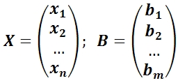
  where ( A|B) Is the main matrix of the system;
  A- extended system matrix;
  X- column of unknowns;
  B- column of free members.
  If the matrix B is not a null matrix ∅, then this system linear equations are called heterogeneous.
  If the matrix B= ∅, then this system of linear equations is called homogeneous. A homogeneous system always has a zero (trivial) solution: x 1 = x 2 =…, x n = 0.
  Joint system of linear equations Is a system of linear equations that has a solution.
  Inconsistent system of linear equations Is a system of linear equations that has no solution.
  A definite system of linear equations Is a system of linear equations that has a unique solution.
  Indefinite system of linear equations Is a system of linear equations that has an infinite set of solutions.
• Systems of n linear equations with n unknowns
  If the number of unknowns is equal to the number of equations, then the matrix is ​​square. The determinant of a matrix is ​​called the main determinant of a system of linear equations and is denoted by the symbol Δ.
  Cramer's method to solve systems n linear equations with n unknown.
  Cramer's rule.
  If the main determinant of a system of linear equations is not equal to zero, then the system is consistent and defined, and the only solution is calculated by Cramer's formulas:
  where Δ i - determinants obtained from the main determinant of the system Δ by replacing i th column per free member column. ...
• Systems of m linear equations with n unknowns
  Kronecker - Capelli theorem.
  
  
  For a given system of linear equations to be consistent, it is necessary and sufficient that the rank of the matrix of the system be equal to the rank of the extended matrix of the system, rang (Α) = rang (Α | B).
  If rang (Α) ≠ rang (Α | B), then the system certainly has no solutions.
  If rang (Α) = rang (Α | B), then two cases are possible:
  1) rang (Α) = n(to the number of unknowns) - the solution is unique and can be obtained by Cramer's formulas;
  2) rang (Α)< n - there are infinitely many solutions.
• Gauss method for solving systems of linear equations
  
  
  Let's compose an expanded matrix ( A|B) of a given system of coefficients at unknown and right-hand sides.
  The Gauss method or the method of eliminating unknowns consists in reducing the extended matrix ( A|B) with the help of elementary transformations over its rows to the diagonal form (to the upper triangular form). Returning to the system of equations, all unknowns are determined.
  Elementary transformations over strings include the following:
  1) swapping two lines;
  2) multiplying a string by a number other than 0;
  3) adding to the string another string multiplied by an arbitrary number;
  4) throwing out the null string.
  The expanded matrix, reduced to a diagonal form, corresponds linear system, which is equivalent to the given one, the solution of which is not difficult. ...
• System of homogeneous linear equations.
  A homogeneous system looks like:
  
  it corresponds to the matrix equation A X = 0.
  1) A homogeneous system is always compatible, since r (A) = r (A | B), there is always a zero solution (0, 0,…, 0).
  2) For a homogeneous system to have a nonzero solution, it is necessary and sufficient that r = r (A)< n , which is equivalent to Δ = 0.
  3) If r< n , then deliberately Δ = 0, then free unknowns arise c 1, c 2, ..., c n-r, the system has nontrivial solutions, and there are infinitely many of them.
  4) General solution X at r< n can be written in matrix form as follows:
  X = c 1 X 1 + c 2 X 2 +… + c n-r X n-r,
  where are the solutions X 1, X 2, ..., X n-r form a fundamental system of decisions.
  5) The fundamental system of solutions can be obtained from the general solution of a homogeneous system:
  
  ,
  if the parameter values ​​are sequentially assumed to be (1, 0,…, 0), (0, 1,…, 0),…, (0, 0,…, 1).
  Decomposition of the general solution in terms of the fundamental system of solutions Is a record of a general solution in the form of a linear combination of solutions belonging to the fundamental system.
  Theorem... In order for the system of linear homogeneous equations has a nonzero solution, it is necessary and sufficient that Δ ≠ 0.
  So, if the determinant Δ ≠ 0, then the system has a unique solution.
  If Δ ≠ 0, then the system of linear homogeneous equations has an infinite set of solutions.
  Theorem... For a homogeneous system to have a nonzero solution, it is necessary and sufficient that r (A)< n .
  Proof:
  1) r can't be more n(the rank of the matrix does not exceed the number of columns or rows);
  2) r< n since if r = n, then the main determinant of the system is Δ ≠ 0, and, according to Cramer's formulas, there is a unique trivial solution x 1 = x 2 =… = x n = 0, which contradicts the condition. Means, r (A)< n .
  Consequence... In order for a homogeneous system n linear equations with n unknowns has a nonzero solution, it is necessary and sufficient that Δ = 0.

A system of linear equations is a union of n linear equations, each of which contains k variables. It is written like this:

Many people, first encountering higher algebra, mistakenly believe that the number of equations must necessarily coincide with the number of variables. In school algebra, this usually happens, but for higher algebra this, generally speaking, is not true.

A solution to a system of equations is a sequence of numbers (k 1, k 2, ..., k n), which is a solution to each equation in the system, i.e. when substituted into this equation instead of variables x 1, x 2, ..., x n gives the correct numerical equality.

Accordingly, solving a system of equations means finding the set of all its solutions or proving that this set is empty. Since the number of equations and the number of unknowns may not coincide, three cases are possible:

1. The system is inconsistent, i.e. the set of all solutions is empty. A fairly rare case that is easily detected regardless of the method used to solve the system.
2. The system is consistent and defined, i.e. has exactly one solution. The classic version, well known since school.
3. The system is consistent and undefined, i.e. has infinitely many solutions. This is the toughest option. It is not enough to point out that "the system has an infinite set of solutions" - it is necessary to describe how this set is arranged.

A variable x i is called allowed if it is included in only one equation of the system, and with a coefficient 1. In other words, in the remaining equations, the coefficient at the variable x i must be equal to zero.

If in each equation we choose one allowed variable, we get a set of allowed variables for the entire system of equations. The system itself, written in this form, will also be called permitted. Generally speaking, one and the same initial system can be reduced to different allowed ones, but now we do not care. Here are examples of permitted systems:

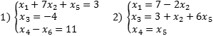
Both systems are allowed with respect to the variables x 1, x 3 and x 4. However, with the same success it can be argued that the second system is allowed with respect to x 1, x 3 and x 5. It is enough to rewrite the most recent equation as x 5 = x 4.

Let us now consider a more general case. Let us assume that we have k variables, of which r are allowed. Then two cases are possible:

1. The number of allowed variables r is equal to the total number of variables k: r = k. We obtain a system of k equations in which r = k allowed variables. Such a system is joint and definite, since x 1 = b 1, x 2 = b 2, ..., x k = b k;
2. The number of allowed variables r is less than the total number of variables k: r< k . Остальные (k − r ) переменных называются свободными - они могут принимать любые значения, из которых легко вычисляются разрешенные переменные.

So, in the above systems, the variables x 2, x 5, x 6 (for the first system) and x 2, x 5 (for the second) are free. The case when there are free variables is best formulated as a theorem:

Please note: this is a very important point! Depending on how you write the resulting system, the same variable can be both allowed and free. Most of the tutors higher mathematics it is recommended to write out variables in lexicographic order, i.e. ascending index. However, you don't have to follow this advice at all.

Theorem. If in a system of n equations the variables x 1, x 2, ..., x r are allowed, and x r + 1, x r + 2, ..., x k are free, then:

1. If we set the values ​​to free variables (xr + 1 = tr + 1, xr + 2 = tr + 2, ..., xk = tk) and then find the values ​​x 1, x 2, ..., xr, we get one of solutions.
2. If in two solutions the values ​​of the free variables coincide, then the values ​​of the allowed variables also coincide, i.e. solutions are equal.

What is the meaning of this theorem? To obtain all solutions of the resolved system of equations, it is sufficient to select free variables. Then, assigning to free variables different meanings, we will receive ready-made solutions. That's all - in this way you can get all the solutions of the system. There are no other solutions.

Conclusion: the resolved system of equations is always consistent. If the number of equations in the resolved system is equal to the number of variables, the system will be definite; if less, it will be indefinite.

And everything would be fine, but the question arises: how to get the resolved one from the original system of equations? For this there is

Systems of linear equations. Lecture 6.

Systems of linear equations.

Basic concepts.

View system

called system - linear equations with unknowns.

The numbers,, are called system coefficients.

The numbers are called free members of the system, – system variables... Matrix

called the main matrix of the system and the matrix

– matrix extended system... Matrices - Columns

And correspondingly matrices of free members and unknowns of the system... Then, in matrix form, the system of equations can be written in the form. System solution is called the values ​​of the variables, when substituted, all the equations of the system turn into true numerical equalities. Any solution to the system can be represented in the form of a matrix - a column. Then matrix equality is valid.

The system of equations is called joint if it has at least one solution and inconsistent if it has no solution.

To solve a system of linear equations means to find out whether it is compatible and, in the case of compatibility, to find its general solution.

The system is called homogeneous if all of its free members are equal to zero. A homogeneous system is always compatible, since it has a solution

The Kronecker - Copelli theorem.

The answer to the question of the existence of solutions to linear systems and their uniqueness allows us to obtain the following result, which can be formulated in the form of the following statements regarding the system of linear equations with unknowns

(1)

Theorem 2... The system of linear equations (1) is consistent if and only if the rank of the main matrix is ​​equal to the rank of the extended (.

Theorem 3... If the rank of the main matrix of a joint system of linear equations is equal to the number of unknowns, then the system has a unique solution.

Theorem 4... If the rank of the main matrix of a compatible system is less than the number of unknowns, then the system has an infinite set of solutions.

System solution rules.

3. Find the expression of the main variables in terms of free ones and get the general solution of the system.

4. By giving arbitrary values ​​to free variables, all the values ​​of the principal variables are obtained.

Methods for solving systems of linear equations.

Inverse matrix method.

moreover, that is, the system has a unique solution. Let us write the system in matrix form

where , , .

Let's multiply both sides matrix equation left to matrix

Since, then we obtain, whence we obtain the equality for finding the unknowns

Example 27. Using the inverse matrix method, solve the system of linear equations

Solution. Let us denote by the main matrix of the system

.

Let, then we find the solution by the formula.

Let's calculate.

Since, then the system has a unique solution. Find all algebraic complements

, ,

, ,

, ,

, ,

Thus

.

Let's check

.

The inverse matrix was found correctly. From here, using the formula, we find the matrix of variables.

.

Comparing the values ​​of the matrices, we get the answer:.

Cramer's method.

Let a system of linear equations with unknowns be given

moreover, that is, the system has a unique solution. Let us write down the solution of the system in matrix form or

We denote

. . . . . . . . . . . . . . ,

Thus, we obtain formulas for finding the values ​​of unknowns, which are called Cramer's formulas.

Example 28. Solve the following system of linear equations by Cramer's method .

Solution. Let us find the determinant of the main matrix of the system

.

Since, then, the system has a single solution.

Let us find the remaining determinants for Cramer's formulas

,

,

.

Using Cramer's formulas, we find the values ​​of the variables

Gauss method.

The method consists in sequential elimination of variables.

Let a system of linear equations with unknowns be given.

The Gaussian solution process consists of two stages:

At the first stage, the expanded matrix of the system is reduced using elementary transformations to a stepwise form

,

where, to which the system corresponds

After that the variables are considered free and in each equation are transferred to the right-hand side.

At the second stage, a variable is expressed from the last equation, the resulting value is substituted into the equation. From this equation

variable is expressed. This process continues until the first equation. The result is an expression of the main variables in terms of free variables .

Example 29. Solve the following system using the Gaussian method

Solution. Let us write out the extended matrix of the system and reduce it to a stepped form

.

Because more than the number of unknowns, then the system is consistent and has an infinite set of solutions. Let us write the system for the stepped matrix

The determinant of the extended matrix of this system, composed of the first three columns, is not equal to zero, therefore, it is considered basic. Variables

They will be basic and the variable will be free. We transfer it in all equations to the left side

From the last equation we express

Substituting this value in the penultimate second equation, we get

where ... Substituting the values ​​of the variables and into the first equation, we find ... We write the answer in the following form

WITH n unknowns is a system of the form:

where a ij and b i (i = 1, ..., m; b = 1, ..., n) are some known numbers, and x 1, ..., x n- unknown numbers. In the designation of the coefficients a ij index i determines the number of the equation, and the second j- the number of the unknown who has this coefficient.

Homogeneous system - when all free terms of the system are equal to zero ( b 1 = b 2 =… = b m = 0), the opposite situation is heterogeneous system.

Square system - when the number m equations is equal to the number n unknown.

System solution- aggregate n numbers c 1, c 2, ..., c n, such that the substitution of all c i instead of x i into a system transforms all its equations into identities.

Collaborative system - when the system has at least 1 solution, and inconsistent system when the system has no solutions.

A joint system of this type (as given above, let it be (1)) can have one or more solutions.

Solutions c 1 (1), c 2 (1), ..., c n (1) and c 1 (2), c 2 (2), ..., c n (2) joint system of type (1) will be various, when even 1 of the equalities fails:

c 1 (1) = c 1 (2), c 2 (1) = c 2 (2), ..., c n (1) = c n (2).

A joint system of type (1) will a certain when she has only one solution; when the system has at least 2 different solutions, it becomes underdetermined... When there are more equations than unknowns, the system is redefined.

The coefficients for unknowns are written as a matrix:

It is called system matrix.

The numbers on the right-hand sides of the equations b 1, ..., b m are free members.

The aggregate n numbers c 1, ..., c n is a solution to this system when all the equations of the system turn into equality after substituting the numbers c 1, ..., c n instead of the corresponding unknowns x 1, ..., x n.

When solving a system of linear equations, 3 options may arise:

1. The system has only one solution.

2. The system has an endless number of solutions. For example,. The solution to this system will be all pairs of numbers that differ in sign.

3. The system has no solutions. For example, if a solution existed, then x 1 + x 2 would equal 0 and 1 at the same time.

Methods for solving systems of linear equations.

Direct methods give an algorithm for finding the exact solution SLAU(systems of linear algebraic equations). And if the accuracy was absolute, they would find it. A real electro-computer, of course, works with an error, so the solution will be approximate.